Estimating the position and orientation of 3D objects is one of the core problems in computer vision applications that involve object-level perception, such as augmented reality and robotic manipulation. In these applications, it is important to know the 3D position of objects in the world, either to directly affect them, or to place simulated objects correctly around them. While there has been much research on this topic using machine learning (ML) techniques, especially Deep Nets, most have relied on the use of depth sensing devices, such as the Kinect, which give direct measurements of the distance to an object. For objects that are shiny or transparent, direct depth sensing does not work well. For example, the figure below includes a number of objects (left), two of which are transparent stars. A depth device does not find good depth values for the stars, and gives a very poor reconstruction of the actual 3D points (right).

Left: RGB image of transparent objects.  Right: A four-panel image showing the reconstructed depth for the scene on the left.The top row includes depth images and the bottom row presents the 3D point cloud. The left panels were reconstructed using a depth camera and the right panels are output from the ClearGrasp model.  Note that although ClearGrasp inpaints the depth of the stars, it mistakes the actual depth of the rightmost one.

One solution to this problem, such as that proposed by ClearGrasp, is to use a deep neural network to inpaint the corrupted depth map of the transparent objects. Given a single RGB-D image of transparent objects, ClearGrasp uses deep convolutional networks to infer surface normals, masks of transparent surfaces, and occlusion boundaries, which it uses to refine the initial depth estimates for all transparent surfaces in the scene (far right in the figure above). This approach is very promising, and allows scenes with transparent objects to be processed by pose-estimation methods that rely on depth.  But inpainting can be tricky, especially when trained completely with synthetic images, and can still result in errors in depth.

In “KeyPose: Multi-View 3D Labeling and Keypoint Estimation for Transparent Objects”, presented at CVPR 2020 in collaboration with the Stanford AI Lab, we describe an ML system that estimates the depth of transparent objects by directly predicting 3D keypoints. To train the system we gather a large real-world dataset of images of transparent objects in a semi-automated way, and efficiently label their pose using 3D keypoints selected by hand. We then train deep models (called KeyPose) to estimate the 3D keypoints end-to-end from monocular or stereo images, without explicitly computing depth. The models work on objects both seen and unseen during training, for both individual objects and categories of objects. While KeyPose can work with monocular images, the extra information available from stereo images allows it to improve its results by a factor of two over monocular image input, with typical errors from 5 mm to 10 mm, depending on the objects. It substantially improves over state-of-the-art in pose estimation for these objects, even when competing methods are provided with ground truth depth. We are releasing the dataset of keypoint-labeled transparent objects for use by the research community.

Real-World Transparent Object Dataset with 3D Keypoint Labels
To facilitate gathering large quantities of real-world images, we set up a robotic data-gathering system in which a robot arm moves through a trajectory while taking video with two devices, a stereo camera and the Kinect Azure depth camera.

Automated image sequence capture using a robot arm with a stereo camera and an Azure Kinect device.

The AprilTags on the target enable accurate tracing of the pose of the cameras. By hand-labelling only a few images in each video with 2D keypoints, we can extract 3D keypoints for all frames of the video using multi-view geometry, thus increasing the labelling efficiency by a factor of 100.

We captured imagery for 15 different transparent objects in five categories, using 10 different background textures and four different poses for each object, yielding a total of 600 video sequences comprising 48k stereo and depth images. We also captured the same images with an opaque version of the object, to provide accurate ground truth depth images. All the images are labelled with 3D keypoints. We are releasing this dataset of real-world images publicly, complementing the synthetic ClearGrasp dataset with which it shares similar objects.

KeyPose Algorithm Using Early Fusion Stereo
The idea of using stereo images directly for keypoint estimation was developed independently for this project; it has also appeared recently in the context of hand-tracking. The diagram below shows the basic idea: the two images from a stereo camera are cropped around the object and fed to the KeyPose network, which predicts a sparse set of 3D keypoints that represent the 3D pose of the object. The network is trained using supervision from the labelled 3D keypoints.

One of the key aspects of stereo KeyPose is the use of early fusion to intermix the stereo images, and allow the network to implicitly compute disparity, in contrast to late fusion, in which keypoints are predicted for each image separately, and then combined. As shown in the diagram below, the output of KeyPose is a 2D keypoint heatmap in the image plane along with a disparity (i.e., inverse depth) heatmap for each keypoint. The combination of these two heatmaps yields the 3D coordinate of the keypoint, for each keypoint.

Keypose system diagram. Stereo images are passed to a CNN model to produce a probability heatmap for each keypoint.  This heatmap yields 2D image coordinates U,V for the keypoint.  The CNN model also produces a disparity (inverse depth) heatmap for each keypoint, which when combined with the U,V coordinates, gives a 3D position (X,Y,Z).

When compared to late fusion or to monocular input, early fusion stereo typically is twice as accurate.

Results
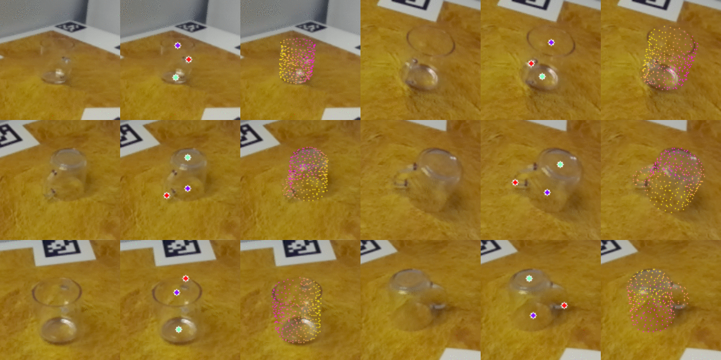
The images below show qualitative results of KeyPose on individual objects. On the left is one of the original stereo images; in the middle are the predicted 3D keypoints projected onto the image. On the right, we visualize points from a 3D model of the bottle, placed at the pose determined by the predicted 3D keypoints. The network is efficient and accurate, predicting keypoints with an MAE of 5.2 mm for the bottle and 10.1 mm for the mug using just 5 ms on a standard GPU.

The following table shows results for KeyPose on category-level estimation. The test set used a background texture not seen by the training set. Note that the MAE varies from 5.8 mm to 9.9 mm, showing the accuracy of the method.

Quantitative comparison of KeyPose with the state-of-the-art DenseFusion system, on category-level data. We provide DenseFusion with two versions of depth, one from the transparent objects, and one from opaque objects. <2cm is the percent of estimates with errors less than 2 cm. MAE is the mean absolute error of the keypoints, in mm.

For a complete accounting of quantitative results, as well as, ablation studies, please see the paper and supplementary materials and the KeyPose website.

Conclusion
This work shows that it is possible to accurately estimate the 3D pose of transparent objects from RGB images without reliance on depth images. It validates the use of stereo images as input to an early fusion deep net, where the network is trained to extract sparse 3D keypoints directly from the stereo pair. We hope the availability of an extensive, labelled dataset of transparent objects will help to advance the field. Finally, while we used semi-automatic methods to efficiently label the dataset, we hope to employ self-supervision methods in future work to do away with manual labelling.

Acknowledgements
I want to thank my co-authors, Xingyu Liu of Stanford University, and Rico Jonschkowski and Anelia Angelova; as well the many who helped us through discussions during the project and paper writing, including Andy Zheng, Shuran Song, Vincent Vanhoucke, Pete Florence, and Jonathan Tompson.

Flooding is the most common natural disaster on the planet, affecting the lives of hundreds of millions of people around the globe and causing around $10 billion in damages each year. Building on our work in previous years, earlier this week we announced some of our recent efforts to improve flood forecasting in India and Bangladesh, expanding coverage to more than 250 million people, and providing unprecedented lead time, accuracy and clarity.

To enable these breakthroughs, we have devised a new approach for inundation modeling, called a morphological inundation model, which combines physics-based modeling with machine learning (ML) to create more accurate and scalable inundation models in real-world settings. Additionally, our new alert-targeting model allows identifying areas at risk of flooding at unprecedented scale using end-to-end machine learning models and data that is publicly available globally. In this post, we also describe developments for the next generation of flood forecasting systems, called HydroNets (presented at ICLR AI for Earth Sciences and EGU this year), which is a new architecture specially built for hydrologic modeling across multiple basins, while still optimizing for accuracy at each location.

Forecasting Water Levels
The first step in a flood forecasting system is to identify whether a river is expected to flood. Hydrologic models (or gauge-to-gauge models) have long been used by governments and disaster management agencies to improve the accuracy and extend the lead time of their forecasts. These models receive inputs like precipitation or upstream gauge measurements of water level (i.e., the absolute elevation of the water above sea level) and output a forecast for the water level (or discharge) in the river at some time in the future.

The hydrologic model component of the flood forecasting system described in this week’s Keyword post doubled the lead time of flood alerts for areas covering more than 75 million people. These models not only increase lead time, but also provide unprecedented accuracy, achieving an R² score of more than 99% across all basins we cover, and predicting the water level within a 15 cm error bound more than 90% of the time. Once a river is predicted to reach flood level, the next step in generating actionable warnings is to convert the river level forecast into a prediction for how the floodplain will be affected.

Morphological Inundation Modeling
In prior work, we developed high quality elevation maps based on satellite imagery, and ran physics-based models to simulate water flow across these digital terrains, which allowed warnings with unprecedented resolution and accuracy in data-scarce regions. In collaboration with our satellite partners, Airbus, Maxar and Planet, we have now expanded the elevation maps to cover hundreds of millions of square kilometers. However, in order to scale up the coverage to such a large area while still retaining high accuracy, we had to re-invent how we develop inundation models.

Inundation modeling estimates what areas will be flooded and how deep the water will be. This visualization conceptually shows how inundation could be simulated, how risk levels could be defined (represented by red and white colors), and how the model could be used to identify areas that should be warned (green dots).

Inundation modeling at scale suffers from three significant challenges. Due to the large areas involved and the resolution required for such models, they necessarily have high computational complexity. In addition, most global elevation maps don’t include riverbed bathymetry, which is important for accurate modeling. Finally, the errors in existing data, which may include gauge measurement errors, missing features in the elevation maps, and the like, need to be understood and corrected. Correcting such problems may require collecting additional high-quality data or fixing erroneous data manually, neither of which scale well.

Our new approach to inundation modeling, which we call a morphological model, addresses these issues by using several innovative tricks. Instead of modeling the complex behaviors of water flow in real time, we compute modifications to the morphology of the elevation map that allow one to simulate the inundation using simple physical principles, such as those describing hydrostatic systems.

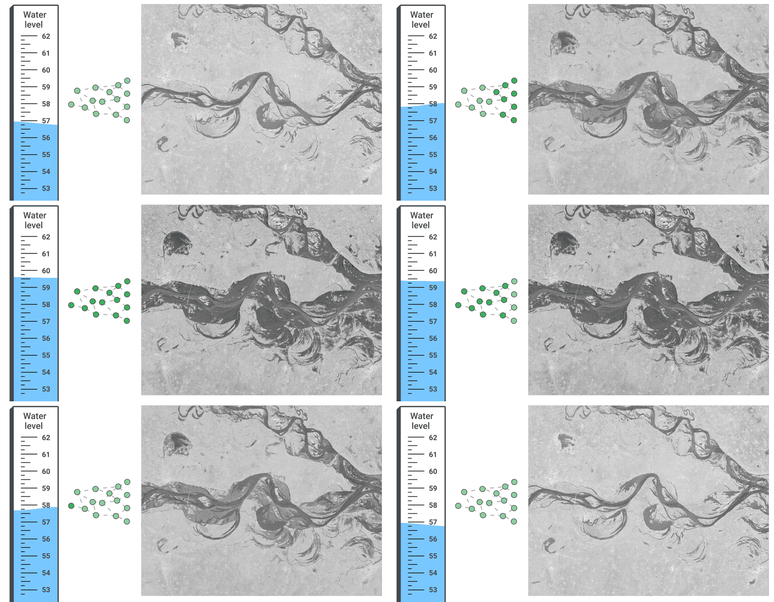
First, we train a pure-ML model (devoid of physics-based information) to estimate the one-dimensional river profile from gauge measurements. The model takes as input the water level at a specific point on the river (the stream gauge) and outputs the river profile, which is the water level at all points in the river. We assume that if the gauge increases, the water level increases monotonically, i.e., the water level at other points in the river increases as well. We also assume that the absolute elevation of the river profile decreases downstream (i.e., the river flows downhill).

We then use this learned model and some heuristics to edit the elevation map to approximately “cancel out” the pressure gradient that would exist if that region were flooded. This new synthetic elevation map provides the foundation on which we model the flood behavior using a simple flood-fill algorithm. Finally, we match the resulting flooded map to the satellite-based flood extent with the original stream gauge measurement.

This approach abandons some of the realistic constraints of classical physics-based models, but in data scarce regions where existing methods currently struggle, its flexibility allows the model to automatically learn the correct bathymetry and fix various errors to which physics-based models are sensitive. This morphological model improves accuracy by 3%, which can significantly improve forecasts for large areas, while also allowing for much more rapid model development by reducing the need for manual modeling and correction.

Alert targeting
Many people reside in areas that are not covered by the morphological inundation models, yet access to accurate predictions are still urgently needed. To reach this population and to increase the impact of our flood forecasting models, we designed an end-to-end ML-based approach, using almost exclusively data that is globally publicly available, such as stream gauge measurements, public satellite imagery, and low resolution elevation maps. We train the model to use the data it is receiving to directly infer the inundation map in real time.

A direct ML approach from real-time measurements to inundation.

This approach works well “out of the box” when the model only needs to forecast an event that is within the range of events previously observed. Extrapolating to more extreme conditions is much more challenging. Nevertheless, proper use of existing elevation maps and real-time measurements can enable alerts that are more accurate than presently available for those in areas not covered by the more detailed morphological inundation models. Because this model is highly scalable, we were able to launch it across India after only a few months of work, and we hope to roll it out to many more countries soon.

Improving Water Levels Forecasting
In an effort to continue improving flood forecasting, we have developed HydroNets — a specialized deep neural network architecture built specifically for water levels forecasting — which allows us utilize some exciting recent advances in ML-based hydrology in a real-world operational setting. Two prominent features distinguish it from standard hydrologic models. First, it is able to differentiate between model components that generalize well between sites, such as the modeling of rainfall-runoff processes, and those that are specific to a given site, like the rating curve, which converts a predicted discharge volume into an expected water level. This enables the model to generalize well to different sites, while still fine-tuning its performance to each location. Second, HydroNets takes into account the structure of the river network being modeled, by training a large architecture that is actually a web of smaller neural networks, each representing a different location along the river. This allows neural networks that are modeling upstream sites to pass information encoded in embeddings to models of downstream sites, so that every model can know everything it needs without a drastic increase in parameters.

The animation below illustrates the structure and flow of information in HydroNets. The output from the modeling of upstream sub-basins is combined into a single representation of a given basin state. It is then processed by the shared model component, which is informed by all basins in the network, and passed on to the label prediction model, which calculates the water level (and the loss function). The output from this iteration of the network is then passed on to inform downstream models, and so on.

An illustration of the HydroNets architecture.

We’re incredibly excited about this progress, and are working hard on improving our systems further.

Acknowledgements
This work is a collaboration between the Google Flood Forecasting Initiative, the Google Geo and Crisis Response teams, Google.org and many other research teams at Google, and is part of our AI for Social Good efforts. We would also like to thank the Partnerships and Policy teams.

Posted by Kenny Sulaimon, Product Manager, ML Kit; Chengji Yan and Areeba Abid, Software Engineers, ML Kit

Two months ago we introduced the standalone version of the ML Kit SDK, making it even easier to integrate on-device machine learning into mobile apps. Since then we’ve launched the Digital Ink Recognition API, and also introduced the ML Kit early access program. Our first two early access APIs were Pose Detection and Entity Extraction. We’ve received an overwhelming amount of interest in these new APIs and today, we are thrilled to officially add Pose Detection to the ML Kit lineup.

A New ML Kit API, Pose Detection

Examples of ML Kit Pose Detection

ML Kit Pose Detection is an on-device, cross platform (Android and iOS), lightweight solution that tracks a subject's physical actions in real time. With this technology, building a one-of-a-kind experience for your users is easier than ever.

The API produces a full body 33 point skeletal match that includes facial landmarks (ears, eyes, mouth, and nose), along with hands and feet tracking. The API was also trained on a variety of complex athletic poses, such as Yoga positions.

Skeleton image detailing all 33 landmark points

Under The Hood

Diagram of the ML Kit Pose Detection Pipeline

The power of the ML Kit Pose Detection API is in its ease of use. The API builds on the cutting edge BlazePose pipeline and allows developers to build great experiences on Android and iOS, with little effort. We offer a full body model, support for both video and static image use cases, and have added multiple pre and post processing improvements to help developers get started with only a few lines of code.

The ML Kit Pose Detection API utilizes a two step process for detecting poses. First, the API combines an ultra-fast face detector with a prominent person detection algorithm, in order to detect when a person has entered the scene. The API is capable of detecting a single (highest confidence) person in the scene and requires the face of the user to be present in order to ensure optimal results.

Next, the API applies a full body, 33 landmark point skeleton to the detected person. These points are rendered in 2D space and do not account for depth. The API also contains a streaming mode option for further performance and latency optimization. When enabled, instead of running person detection on every frame, the API only runs this detector when the previous frame no longer detects a pose.

The ML Kit Pose Detection API also features two operating modes, “Fast” and “Accurate”. With the “Fast” mode enabled, you can expect a frame rate of around 30+ FPS on a modern Android device, such as a Pixel 4 and 45+ FPS on a modern iOS device, such as an iPhone X. With the “Accurate” mode enabled, you can expect more stable x,y coordinates on both types of devices, but a slower frame rate overall.

Lastly, we’ve also added a per point “InFrameLikelihood” score to help app developers ensure their users are in the right position and filter out extraneous points. This score is calculated during the landmark detection phase and a low likelihood score suggests that a landmark is outside the image frame.

Real World Applications

Examples of a pushup and squat counter using ML Kit Pose Detection

Keeping up with regular physical activity is one of the hardest things to do while at home. We often rely on gym buddies or physical trainers to help us with our workouts, but this has become increasingly difficult. Apps and technology can often help with this, but with existing solutions, many app developers are still struggling to understand and provide feedback on a user’s movement in real time. ML Kit Pose Detection aims to make this problem a whole lot easier.

The most common applications for Pose detection are fitness and yoga trackers. It’s possible to use our API to track pushups, squats and a variety of other physical activities in real time. These complex use cases can be achieved by using the output of the API, either with angle heuristics, tracking the distance between joints, or with your own proprietary classifier model.

To get you jump started with classifying poses, we are sharing additional tips on how to use angle heuristics to classify popular yoga poses. Check it out here.

Learning to Dance Without Leaving Home

Learning a new skill is always tough, but learning to dance without the aid of a real time instructor is even tougher. One of our early access partners, Groovetime, has set out to solve this problem.

With the power of ML Kit Pose Detection, Groovetime allows users to learn their favorite dance moves from popular short-form dance videos, while giving users automated real time feedback on their technique. You can join their early access beta here.

Groovetime App using ML Kit Pose Detection

Staying Active Wherever You Are

Our Pose Detection API is also helping adidas Training, another one of our early access partners, build a virtual workout experience that will help you stay active no matter where you are. This one-of-a-kind innovation will help analyze and give feedback on the user’s movements, using nothing more than just your phone. Integration into the adidas Training app is still in the early phases of the development cycle, but stay tuned for more updates in the future.

How to get started?

If you would like to start using the Pose Detection API in your mobile app, head over to the developer documentation or check out the sample apps for Android and iOS to see the API in action. For questions or feedback, please reach out to us through one of our community channels.

Most people take for granted the ability to view an object from several different angles, but still recognize that it's the same object— a dog viewed from the front is still a dog when viewed from the side. While people do this naturally, computer scientists need to explicitly enable machines to learn representations that are view-invariant, with the goal of seeking robust data representations that retain information that is useful to downstream tasks.

Of course, in order to learn these representations, manually annotated training data can be used. However, as in many cases such annotations aren’t available, which gives rise to a series of self- and crossmodal supervised approaches that do not require manually annotated training data. Currently, a popular paradigm for training with such data is contrastive multiview learning, where two views of the same scene (for example, different image channels, augmentations of the same image, and video and text pairs) will tend to converge in representation space while two views of different scenes diverge. Despite their success, one important question remains: “If one doesn’t have annotated labels readily available, how does one select the views to which the representations should be invariant?” In other words, how does one identify an object using information that resides in the pixels of the image itself, while still remaining accurate when that image is viewed from disparate viewpoints?

In “What makes for good views for contrastive learning”, we use theoretical and empirical analysis to better understand the importance of view selection, and argue that one should reduce the mutual information between views while keeping task-relevant information intact. To verify this hypothesis, we devise unsupervised and semi-supervised frameworks that learn effective views by aiming to reduce their mutual information. We also consider data augmentation as a way to reduce mutual information, and show that increasing data augmentation indeed leads to decreasing mutual information while improving downstream classification accuracy. To encourage further research in this space, we have open-sourced the code and pre-trained models.

The InfoMin Hypothesis
The goal of contrastive multiview learning is to learn a parametric encoder, whose output representations can be used to discriminate between pairs of views with the same identities, and pairs with different identities. The amount and type of information shared between the views determines how well the resulting model performs on downstream tasks. We hypothesize that the views that yield the best results should discard as much information in the input as possible except for the task relevant information (e.g., object labels), which we call the InfoMin principle.

Consider the example below in which two patches of the same image represent the different “views”. The training objective is to identify that the two views belong to the same image. It is undesirable to have views that share too much information, for example, where low-level color and texture cues can be exploited as “shortcuts” (left), or to have views that share too little information to identify that they belong to the same image (right). Rather, views at the “sweet spot” share the information related to downstream tasks, such as patches corresponding to different parts of the panda for an object classification task (center).

An illustration of three regimes of information captured during contrastive multiview learning. Views should not share too much information (left) or too little information (right), but should find an optimal mix (the “sweet spot”, middle) that maximizes the downstream performance.

A Unified View on Contrastive Learning
We design several sets of experiments to verify the InfoMin hypothesis, motivated by the fact that there are simple ways to control the mutual information shared between views without any supervision. For example, we can sample different patches from the same images, and reduce their mutual information simply by increasing the distance between the patches. Here, we estimate the mutual information using InfoNCE (I_NCE), which is a quantitative measure of the mutual information lower bound._. Indeed, we observe a reverse U-shape curve: as mutual information is reduced, the downstream task accuracy first increases and then begins to decrease.

Downstream classification accuracy on STL-10 (left) and CIFAR-10 (right) by applying linear classifiers on representations learned with contrastive learning. Same as the previous illustration, the views are sampled as different patches from the same images. Increasing the Euclidean distance between patches leads to decreasing mutual information. A reverse U-shape curve between classification accuracy and INCE (patch distance) is observed.

Furthermore, we demonstrate that several state-of-the-art contrastive learning methods (InstDis, MoCo, CMC, PIRL, SimCLR and CPC) can be unified through the perspective of view selection: despite the differences in architecture, objective and engineering details, all recent contrastive learning methods create two views that implicitly follow the InfoMin hypothesis, where the information shared between views are controlled by the strength of data augmentation. Motivated by this, we propose a new set of data augmentations, which outperforms the prior state of the art, SimCLR, by nearly 4% on the ImageNet linear readout benchmark. We also found that transferring our unsupervised pre-trained models to object detection and instance segmentation consistently outperforms ImageNet pre-training.

Learning to Generate Views
In our work, we design unsupervised and semi-supervised methods that synthesize novel views following the InfoMin hypothesis. We learn flow-based models that transfer natural color spaces into novel color spaces, from which we split the channels to get views. For the unsupervised setup, the view generators are optimized to minimize the InfoNCE bound between views. As shown in the results below, we observe a similar reverse U-shape trend while minimizing the InfoNCE bound.

View generators learned by unsupervised (left) and semi-supervised (right) objectives.

To reach the sweet spot without overly minimizing mutual information, we can use the semi-supervised setup and guide the view generator to retain label information. As expected, all learned views are now centered around the sweet spot, no matter what the input color space is.

Code and Pretrained Models
To accelerate research in self-supervised contastive learning, we are excited to share the code and pretrained models of InfoMin with the academic community. They can be found here.

Acknowledgements
The core team includes Yonglong Tian, Chen Sun, Ben Poole, Dilip Krishnan, Cordelia Schmid and Phillip Isola. We would like to thank Kevin Murphy for insightful discussion; Lucas Beyer for feedback on the manuscript; and the Google Cloud team for computation support.

The two-tower neural network model, illustrated above, is a specific type of embedding-based search where queries and database items are mapped to the embedding space by two respective neural networks. In this example the model responds to natural-language queries for a hypothetical literary database.

The goal is to quantize each xi to x̃i = c1 or x̃i = c2. Traditional quantization (left) results in the incorrect ordering of x1 and x2 for this query. Even though our approach (right) chooses centers farther away from the data points, this in fact leads to lower inner product error and higher accuracy.

In the above diagrams, ellipses denote contours of equal loss. In anisotropic vector quantization, error parallel to the original data point x is penalized more.

Recall@k is a commonly used metric for nearest neighbor search accuracy, which measures the proportion of the true nearest k neighbors that are present in an algorithm’s returned k neighbors. ScaNN (upper purple line) consistently achieves superior performance across various points of the speed-accuracy trade-off.

* ScaNN performs similarly well on the other datasets of ann-benchmarks.com, but the website currently shows outdated, lower numbers. See this pull request for more representative performance figures on other datasets. ↩

Left: Sixteen individual tests are required to screen 16 people — only one person’s test is positive, while 15 return negative. Right: Following Dorfman’s procedure, samples are pooled into four groups of four individuals, and tests are executed on the pooled samples. Because only the second group tests positive, 12 individuals are cleared and only those four belonging to the positive group need to be retested. This approach requires only eight tests, instead of the 16 needed for an exhaustive testing campaign.

1. Given a population of n people, an infection state is a binary vector of length n that describes who is infected (marked with a 1), and who is not (marked with a 0). At a certain time, a population is in a given state (most likely a few 1’s and mostly 0’s). The goal of group testing is to identify that state using as few tests as possible. Given a prior belief on the infection rate (the disease is rare) and test results observed so far (if any), we expect that only a small share of those infection states will be plausible. Rather than evaluating the plausibility of all 2ⁿ possible states (an extremely large number even for small n), we resort to a more efficient method to sample plausible hypotheses using a sequential Monte Carlo (SMC) sampler. Although quite costly by common standards (a few minutes using a GPU in our experimental setup), we show in this work that SMC samplers remain tractable even for large n, opening new possibilities for group testing. In short, in return for a few minutes of computations, our detectives get an extensive list of thousands of relevant hypotheses that may explain tests observed so far.
   
   
2. Equipped with a relevant list of hypotheses, our strategy proceeds, as detectives would, by selectively gathering additional evidence. If k tests can be carried out at the next iteration, our strategy will propose to test k new groups, which are computed using the framework of Bayesian optimal experimental design. Intuitively, if k=1 and one can only propose a single new group to test, there would be clear advantage in building that group such that its test outcome is as uncertain as possible, i.e., with a probability that it returns positive as close to 50% as possible, given the current set of hypotheses. Indeed, to progress in an investigation, it is best to maximize the surprise factor (or information gain) provided by new test results, as opposed to using them to confirm further what we already hold to be very likely. To generalize that idea to a set of k>1 new groups, we score this surprise factor by computing the mutual information of these “virtual” group tests vs. the distribution of hypotheses. We also consider a more involved approach that computes the expected area under the ROC curve (AUC) one would obtain from testing these new groups using the distribution of hypotheses. The maximization of these two criteria is carried out using a greedy approach, resulting in two group selectors, GMIMAX and GAUCMAX (greedy maximization of mutual information or AUC, respectively).
   

Our group testing framework describes an interaction between a testing environment, the wet_lab, whose pooled test results are used by the sampler to draw thousands of plausible hypotheses on the infection status of all individuals. These hypotheses are then used by an optimization procedure, group_selector, that figures out what groups may be the most relevant to test in order to narrow down on the true infection status. Once formed, these new groups are then tested again, closing the loop. At any point in the procedure, the hypotheses formed by the sampler can be averaged to obtain the average probability of infection for each patient. From these probabilities, a decision on whether a patient is infected or not can be done by thresholding these probabilities at a certain confidence level.

We executed 5000 simulations on a sample population of 70 individuals with an infection rate of 2%. We have assumed sensitivity/specificity values of 85% / 97% for tests with groups of maximal size 10, which are representative of current PCR machines. This figure demonstrates that our approach outperforms the other baselines with as few as 24 tests (up to 8 tests used in 3 cycles), including both adaptive and non-adaptive varieties, and performs significantly better than individual tests (plotted in the sensitivity/specificity plane as a hexagon, requiring 70 tests), highlighting the savings potential offered by group testing. See preprint for other setups.